This page was generated from a Jupyter notebook. Check the source code or download the notebook..

Simple thick lens

This example shows how to create and analyze a simple thick lens as described in the paper ZOSPy: optical ray tracing in Python through OpticStudio. The code resembles the example of the paper with the addition of plotting the analysis results.

Included functionalities

• Sequential mode:

  • Building a simple sequential optical system.

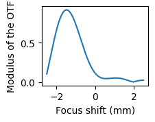
  • Usage of zospy.analyses.mtf.fft_through_focus_mtf to calculate the FFT through focus MTF.

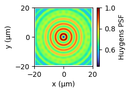
  • Usage of zospy.analyses.psf.huygens_psf() to perform a Huygens PSF analysis.

Warranty and liability

The examples are provided ‘as is’. There is no warranty and rights cannot be derived from them, as is also stated in the general license of this repository.

This example requires to connect to OpticStudio as extension. Also make sure ZOSPy is in sequential mode before running this example.

Import dependencies

from warnings import warn

import matplotlib.pyplot as plt

import zospy as zp

Setup the connection

Initiate the connection to OpticStudio

zos = zp.ZOS()
oss = zos.connect(mode="extension")

Get the primary system and make sure it is an new, empty system

oss.new()

Set up the optical system

1. Alter some system settings regarding the aperture size

oss.SystemData.Aperture.ApertureValue = 10

2. Add the SCHOTT glass catalog if it is not already in use

if "SCHOTT" not in oss.SystemData.MaterialCatalogs.GetCatalogsInUse():
    oss.SystemData.MaterialCatalogs.AddCatalog("SCHOTT")

print("Catalogs currently in use:", " ".join(oss.SystemData.MaterialCatalogs.GetCatalogsInUse()))

Catalogs currently in use: SCHOTT

3. Create an input beam for viewing purposes

input_beam = oss.LDE.InsertNewSurfaceAt(1)  # behind the object surface
input_beam.Thickness = 10

4. Make a 10 mm thick lens with a radius of curvature of 30 mm and material type BK10

front_surface = oss.LDE.GetSurfaceAt(2)
front_surface.Radius = 30
front_surface.Thickness = 10
front_surface.SemiDiameter = 15
front_surface.Material = "BK10"

back_surface = oss.LDE.InsertNewSurfaceAt(3)
back_surface.Radius = -30
back_surface.Thickness = 29
back_surface.SemiDiameter = 15

5. Specify the detector surface

image_surface = oss.LDE.GetSurfaceAt(4)
image_surface.SemiDiameter = 5

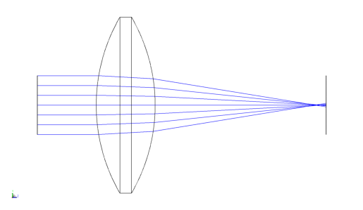
Render the model

draw3d = zp.analyses.systemviewers.viewer_3d(
    oss,
    surface_line_thickness="Thick",
    ray_line_thickness="Thick",
    number_of_rays=7,
    hide_x_bars=True,
    oncomplete="Release",
)

if oss._ZOS.version < (24, 1, 0):
    warn("Exporting the 3D viewer data is not available for this version of OpticStudio.")
else:
    plt.imshow(draw3d.Data)
    plt.axis("off")

Analyze the model and show the results

1. Calculte the FFT through focus MTF and plot it

mtf = zp.analyses.mtf.fft_through_focus_mtf(oss, sampling="512x512", deltafocus=2.5, frequency=3, numberofsteps=51)

fig = plt.figure(figsize=(2, 1.5))
ax = fig.add_subplot(111)
ax.plot(mtf.Data.index, mtf.Data[("Field: 0,0000 (deg)", "Tangential")])
ax.set_xlabel("Focus shift (mm)")
_ = ax.set_ylabel("Modulus of the OTF")

2. Calculate the Huygens PSF and plot it

huygens_psf = zp.analyses.psf.huygens_psf(oss, pupil_sampling="512x512", image_sampling="512x512", normalize=True)

fig = plt.figure(figsize=(2, 1.5))
ax = fig.add_subplot(111)
im = ax.imshow(
    huygens_psf.Data,
    cmap="turbo",
    extent=[
        huygens_psf.Data.columns.values.min(),
        huygens_psf.Data.columns.values.max(),
        huygens_psf.Data.index.values.min(),
        huygens_psf.Data.index.values.max(),
    ],
)
plt.colorbar(im, label="Huygens PSF")
ax.set_xlabel("x (μm)")
ax.set_ylabel("y (μm)")
ax.set_xticks([-20, 0, 20])
_ = ax.set_yticks([-20, 0, 20])