Fitting reverse gradient

Fitting reverse gradient#

In the OpticStudio knowledge base tutorial Modelling of a Shack-Hartmann Sensor for eye aberration evaluation, a reversed eye model is created. That eye model is the reversed version of the finite eye model created in How to model the human eye in OpticStudio. However, the reversed lens gradient is incorrectly inverted. This notebook addresses the fitting of a ‘reverse’ lens gradient for the crystalline lens of the eye, and shows how to correctly determine it.

Included functionalities#

This example does not show ZOSPy functionalities but rather shows how to obtain a reversed lens gradient for a Gradient 3 surface.

Warranty and liability#

The examples are provided ‘as is’. There is no warranty and rights cannot be derived from them, as is also stated in the general license of this repository.

Import dependencies#

[1]:

import matplotlib.pyplot as plt
import numpy as np
from lmfit import Parameters, minimize

First, we create a grad3 function that is equal to the internal function of the OpticStudio Gradient3 surface.

[2]:

def grad3(coords, n0=0, nr2=0, nr4=0, nr6=0, nz1=0, nz2=0, nz3=0) -> np.ndarray:
    """Compute a gradient3 based on radial (r) and axial (z) coordinates.

    Parameters
    ----------
    coords : numpy.ndarray
        A 2D array of shape (n, 2), where the first column represents the radial (r) component and
        the second column represents the axial (z) component. Each row corresponds to a different coordinate pair.
    n0 : float
        The constant term (default is 0).
    nr2 : float
        Coefficient for the r^2 term in the polynomial expansion. Defaults to 0.
    nr4 : float
        Coefficient for the r^4 term in the polynomial expansion. Defaults to 0.
    nr6 : float
        Coefficient for the r^6 term in the polynomial expansion. Defaults to 0.
    nz1 : float
        Coefficient for the z term in the polynomial expansion. Defaults to 0.
    nz2 : float
        Coefficient for the z^2 term in the polynomial expansion. Defaults to 0.
    nz3 : float
        Coefficient for the z^3 term in the polynomial expansion. Defaults to 0.

    Returns
    -------
    result : numpy.ndarray
        A 1D array of length n, where each element corresponds to the evaluated polynomial value for the
        corresponding (r, z) pair in the input coords.
    """
    r = coords[:, 0]
    z = coords[:, 1]
    return n0 + nr2 * r**2 + nr4 * r**4 + nr6 * r**6 + nz1 * z + nz2 * z**2 + nz3 * z**3

Original Lens Gradient#

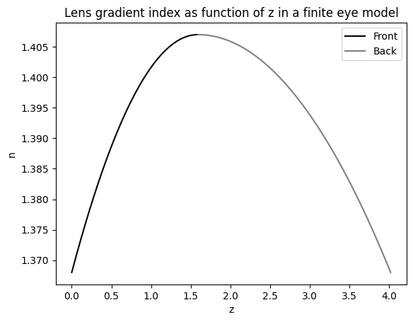
Then, we create the gradient as it would be present in the normal, non-reversed finite eye model.

[3]:

z_front = np.arange(0, 1.60, 0.01)
r_front = np.zeros(z_front.shape)
coords_front = np.array([r_front, z_front]).T
n_front_orig = grad3(coords_front, n0=1.368, nr2=-1.978e-003, nz1=0.049057, nz2=-0.015427)

[4]:

z_back = np.arange(0, 2.44, 0.01)
r_back = np.zeros(z_back.shape)
coords_back = np.array([r_back, z_back]).T
n_back_orig = grad3(coords_back, n0=1.407, nr2=-1.978e-003, nz2=-6.605e-003)

[5]:

fig, ax = plt.subplots()

ax.plot(z_front, n_front_orig, c="k", label="Front")
ax.plot(z_back + z_front.max(), n_back_orig, c="Gray", label="Back")

ax.set_xlabel("z")
ax.set_ylabel("n")

ax.legend()
_ = ax.set_title("Lens gradient index as function of z in a finite eye model")

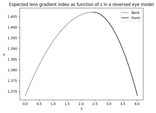
../../_images/examples_Modelling_of_a_Shack-Hartmann_Sensor_for_eye_aberration_evaluation_2_Fitting_reverse_gradient_3_8_0.png

Expected reversed implementation#

The expected reversed gradient would be the gradient curve flipped.

[6]:

n_back_inv_expected = n_back_orig[::-1]
n_front_inv_expected = n_front_orig[::-1]

[7]:

fig, ax = plt.subplots()

ax.plot(z_back, n_back_inv_expected, c="Gray", label="Back")
ax.plot(z_front + z_back.max(), n_front_inv_expected, c="k", label="Front")

ax.set_xlabel("z")
ax.set_ylabel("n")

ax.legend()
_ = ax.set_title("Expected lens gradient index as function of z in a reversed eye model")

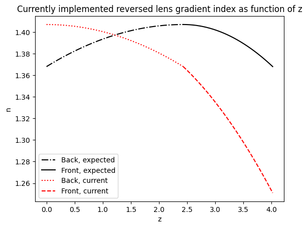
../../_images/examples_Modelling_of_a_Shack-Hartmann_Sensor_for_eye_aberration_evaluation_2_Fitting_reverse_gradient_3_11_0.png

Current reversed implementation#

Now, we generate the same curve based on the Gradient3 constants used in Modelling of a Shack-Hartmann Sensor for eye aberration evaluation.

[8]:

n_back_inv_cur = grad3(coords_back, n0=1.407, nr2=-1.978e-003, nz2=-6.605e-003)
n_front_inv_cur = grad3(coords_front, n0=1.368, nr2=-1.978e-003, nz1=-0.049057, nz2=-0.015427)

[9]:

fig, ax = plt.subplots()

ax.plot(z_back, n_back_inv_expected, c="k", ls="-.", label="Back, expected")
ax.plot(z_front + z_back.max(), n_front_inv_expected, c="k", label="Front, expected")

ax.plot(z_back, n_back_inv_cur, c="red", ls=":", label="Back, current")
ax.plot(z_front + z_back.max(), n_front_inv_cur, c="red", ls="--", label="Front, current")

ax.set_xlabel("z")
ax.set_ylabel("n")

ax.legend()
_ = ax.set_title("Currently implemented reversed lens gradient index as function of z")

../../_images/examples_Modelling_of_a_Shack-Hartmann_Sensor_for_eye_aberration_evaluation_2_Fitting_reverse_gradient_3_15_0.png

New implementation of reverse gradient based on fit#

Now, we use the lmfit module to fit the parameters of the reversed gradient based using the initial non-reversed gradient.

[10]:

def residual(parameters, z, n_orig):
    """
    Compute the residual (absolute difference) between the original and new values of a function defined by `grad3`.

    This function calculates the difference between the original values (`n_orig`) and the new values computed
    by the `grad3` function using a set of polynomial coefficients provided in `parameters`. It evaluates how
    well the new values fit the original data.

    Parameters
    ----------
    parameters : lmfit.Parameters
        A dictionary-like object that holds the values of the polynomial coefficients. The keys are expected to
        be:
        - "n0": The constant term.
        - "nr2": Coefficient for the r^2 term.
        - "nr4": Coefficient for the r^4 term.
        - "nr6": Coefficient for the r^6 term.
        - "nz1": Coefficient for the z term.
        - "nz2": Coefficient for the z^2 term.
        - "nz3": Coefficient for the z^3 term.
    z : numpy.ndarray
        A 2D array of shape (n, 2) containing radial (r) and axial (z) coordinates. This is passed as input to
        the `grad3` function for evaluation.
    n_orig : numpy.ndarray
        A 1D array of original values that represents the target values to compare against the values computed by
        `grad3`.

    Returns
    -------
    residuals : numpy.ndarray
        A 1D array representing the absolute difference between `n_orig` and the values computed by `grad3`.
        This is the residual or error between the original data and the fitted model.
    """
    pars = parameters.valuesdict()
    n_new = grad3(
        z,
        n0=pars["n0"],
        nr2=pars["nr2"],
        nr4=pars["nr4"],
        nr6=pars["nr6"],
        nz1=pars["nz1"],
        nz2=pars["nz2"],
        nz3=pars["nz3"],
    )

    return abs(n_orig - n_new)

Fitting the back surface#

To fit the reversed back surface, we want to know the minimal refractive index of the original back surface, which will be the new n0.

[11]:

n_back_orig.min()

[11]:

np.float64(1.3679981355)

Given the symmetry of the curve, it should be sufficient to solely adjust nz1. Other gradient 3 implementations might require more freedom in the fitting process, and the parameters below can be adjusted accordingly.

[12]:

params = Parameters()
params.add("n0", value=n_back_orig.min(), vary=False)
params.add("nr2", value=-1.978e-003, vary=False)
params.add("nr4", value=0.0, vary=False)
params.add("nr6", value=0.0, vary=False)
params.add("nz1", value=0, vary=True)
params.add("nz2", value=-6.605e-003, vary=False)
params.add("nz3", value=0, vary=False)

Perform the fit.

[13]:

fitres_back = minimize(residual, params=params, args=(coords_back, n_back_inv_expected))
fitres_back.params

[13]:

Parameters
name	value	standard error	relative error	initial value	min	max	vary
n0	1.36799814	0.00000000	(0.00%)	1.3679981355	-inf	inf	False
nr2	-0.00197800	0.00000000	(0.00%)	-0.001978	-inf	inf	False
nr4	0.00000000	0.00000000		0.0	-inf	inf	False
nr6	0.00000000	0.00000000		0.0	-inf	inf	False
nz1	0.03210030	2.4726e-16	(0.00%)	0	-inf	inf	True
nz2	-0.00660500	0.00000000	(0.00%)	-0.006605	-inf	inf	False
nz3	0.00000000	0.00000000		0	-inf	inf	False

Create the resulting gradient.

[14]:

n_back_inv_fit = grad3(
    coords_back,
    n0=fitres_back.params["n0"].value,
    nr2=fitres_back.params["nr2"].value,
    nr4=fitres_back.params["nr4"].value,
    nr6=fitres_back.params["nr6"].value,
    nz1=fitres_back.params["nz1"].value,
    nz2=fitres_back.params["nz2"].value,
    nz3=fitres_back.params["nz3"].value,
)

Fitting the front surface#

Same process as the back surface, including the same reasoning for the fit parameters. The new n0 should however be the maximal refractive index of the front surface.

[15]:

n_front_orig.max()

[15]:

np.float64(1.4069996313000002)

[16]:

params = Parameters()
params.add("n0", value=n_front_orig.max(), vary=False)
params.add("nr2", value=-1.978e-003, vary=False)
params.add("nr4", value=0.0, vary=False)
params.add("nr6", value=0.0, vary=False)
params.add("nz1", value=0.049057, vary=True)
params.add("nz2", value=-0.015427, vary=False)
params.add("nz3", value=0, vary=False)

[17]:

fitres_front = minimize(residual, params=params, args=(coords_front, n_front_inv_expected))
fitres_front.params

[17]:

Parameters
name	value	standard error	relative error	initial value	min	max	vary
n0	1.40699963	0.00000000	(0.00%)	1.4069996313000002	-inf	inf	False
nr2	-0.00197800	0.00000000	(0.00%)	-0.001978	-inf	inf	False
nr4	0.00000000	0.00000000		0.0	-inf	inf	False
nr6	0.00000000	0.00000000		0.0	-inf	inf	False
nz1	8.6000e-07	1.5082e-14	(0.00%)	0.049057	-inf	inf	True
nz2	-0.01542700	0.00000000	(0.00%)	-0.015427	-inf	inf	False
nz3	0.00000000	0.00000000		0	-inf	inf	False

[18]:

n_front_inv_fit = grad3(
    coords_front,
    n0=fitres_front.params["n0"].value,
    nr2=fitres_front.params["nr2"].value,
    nr4=fitres_front.params["nr4"].value,
    nr6=fitres_front.params["nr6"].value,
    nz1=fitres_front.params["nz1"].value,
    nz2=fitres_front.params["nz2"].value,
    nz3=fitres_front.params["nz3"].value,
)

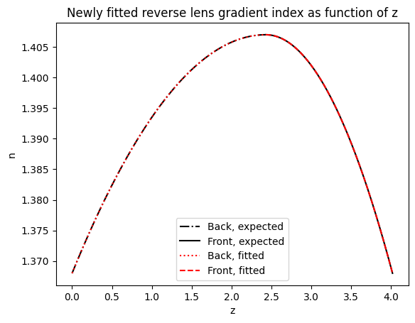
Fitting results#

[19]:

fig, ax = plt.subplots()

ax.plot(z_back, n_back_inv_expected, c="k", ls="-.", label="Back, expected")
ax.plot(z_front + z_back.max(), n_front_inv_expected, c="k", label="Front, expected")

ax.plot(z_back, n_back_inv_fit, c="red", ls=":", label="Back, fitted")
ax.plot(z_front + z_back.max(), n_front_inv_fit, c="red", ls="--", label="Front, fitted")

ax.set_xlabel("z")
ax.set_ylabel("n")

ax.legend()
_ = ax.set_title("Newly fitted reverse lens gradient index as function of z")

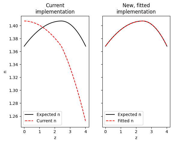
../../_images/examples_Modelling_of_a_Shack-Hartmann_Sensor_for_eye_aberration_evaluation_2_Fitting_reverse_gradient_3_35_0.png

Comparison with original implementation#

Now we overlay both the original reversed lens gradient and the newly fitted reversed lens gradient over the expected reversed lens gradient, showing that the original reversed gradient matches poorly and the newly fitted one matches well.

[20]:

fig, ax = plt.subplots(ncols=2, sharex=True, sharey=True)

ax[0].plot(z_back, n_back_inv_expected, c="k", label="Expected n")
ax[0].plot(z_front + z_back.max(), n_front_inv_expected, c="k")

ax[0].plot(z_back, n_back_inv_cur, c="red", ls="--", label="Current n")
ax[0].plot(z_front + z_back.max(), n_front_inv_cur, c="red", ls="--")

ax[1].plot(z_back, n_back_inv_expected, c="k", label="Expected n")
ax[1].plot(z_front + z_back.max(), n_front_inv_expected, c="k")

ax[1].plot(z_back, n_back_inv_fit, c="red", ls="--", label="Fitted n")
ax[1].plot(z_front + z_back.max(), n_front_inv_fit, c="red", ls="--")

ax[0].set_xlabel("z")
ax[1].set_xlabel("z")
ax[0].set_ylabel("n")

ax[0].legend()
ax[1].legend()

ax[0].set_title("Current\nimplementation")
ax[1].set_title("New, fitted\nimplementation")

[20]:

Text(0.5, 1.0, 'New, fitted\nimplementation')

../../_images/examples_Modelling_of_a_Shack-Hartmann_Sensor_for_eye_aberration_evaluation_2_Fitting_reverse_gradient_3_37_1.png