Polarization prism with total internal reflection#
This example shows how to perform and subsequently plot a polarization analysis in a prisim with total internal reflection. This notebook depends on the example file “Prism using total internal reflection.zmx“, which is also supplied.
Included functionalities#
Sequential mode:
Usage of
zospy.analyses.polarization.PolarizationTransmissionto perform a polarization transmission analysis.Usage of
zospy.analyses.polarization.PolarizationPupilMapto calculate the polarization pupil map.
Warranty and liability#
The examples are provided ‘as is’. There is no warranty and rights cannot be derived from them, as is also stated in the general license of this repository.
Import dependencies#
[1]:
from warnings import warn

import matplotlib.pyplot as plt
import numpy as np

import zospy as zp
Input values#
[2]:
# Input Jones Vector
jx = 1
jy = 1
x_phase = 0
y_phase = 0
Connect to OpticStudio in standalone mode#
[3]:
zos = zp.ZOS()
oss = zos.connect(mode="standalone")
Load the optical system#
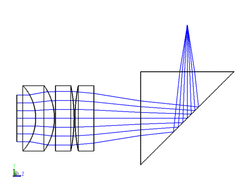
Load the example file ‘Prism using total internal reflection’.
[4]:
# OpticStudio requires absolute paths, but ZOSPy can handle relative paths
oss.load("Prism using total internal reflection.zmx")
Render the model#
To render the model, we use the zospy.analyses.systemviewers.Viewer3D function. For this system, zospy.analyses.systemviewers.CrossSection cannot be used because the system is not rotationally symmetric.
[5]:
draw3d = zp.analyses.systemviewers.Viewer3D(
    surface_line_thickness="Thick",
    rays_line_thickness="Thick",
    number_of_rays=7,
    hide_x_bars=True,
).run(oss)

if zos.version < (24, 1, 0):
    warn("Exporting the 3D viewer data is not available for this version of OpticStudio.")
else:
    plt.imshow(draw3d.data)
    plt.axis("off")
Transmission analysis#
Run the Transmission analysis from zospy.analyses.polarization.transmission.
[6]:
result_transmission = zp.analyses.polarization.PolarizationTransmission(
    jx=jx, jy=jy, x_phase=x_phase, y_phase=y_phase, sampling="64x64"
).run(oss)


print("Field position     Transmission")

for transmission in result_transmission.data.field_transmissions:
    print(
        f"{transmission.field_pos.value} {transmission.field_pos.unit:<14} {transmission.total_transmission * 100:.2f}%"
    )
Field position     Transmission
0.0 deg            64.18%
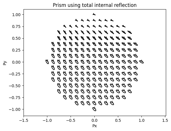
Get a polarization map using zospy.analyses.polarization.PolarizationPupilMap
[7]:
result_pupil_map = zp.analyses.polarization.PolarizationPupilMap(
    jx=jx, jy=jy, x_phase=x_phase, y_phase=y_phase, sampling="17x17"
).run(oss)
df = result_pupil_map.data.pupil_map

print(df)
        Px     Py        Ex        Ey  Intensity  Phase (Deg)  Orientation
0   -1.000  0.000  0.478226  0.673308   0.682044   137.096154   122.267525
1   -0.875 -0.375  0.505769  0.668042   0.702082   134.067624   123.969140
2   -0.875 -0.250  0.501666  0.666814   0.696309  -225.063934   123.893391
3   -0.875 -0.125  0.496899  0.665856   0.690273  -223.867939   123.809086
4   -0.875  0.000  0.491385  0.665160   0.683897  -222.250933   123.722118
..     ...    ...       ...       ...        ...          ...          ...
192  0.875  0.000  0.672867  0.476981   0.680261  -222.668754   147.755937
193  0.875  0.125  0.678455  0.475828   0.686713  -220.284484   147.700755
194  0.875  0.250  0.684247  0.474248   0.693105  -217.117400   147.589012
195  0.875  0.375  0.690386  0.472140   0.699549   147.216066   147.420181
196  1.000  0.000  0.683282  0.457999   0.676638   136.423377   149.777610

[197 rows x 7 columns]
Plot the pupil map
[8]:
xy_length = len(np.unique(df["Px"]))

for i in range(len(df)):
    # E-field coordinates
    phi = np.linspace(0, 2 * np.pi) - np.pi / 3
    Ex = np.real(df["Ex"][i] * np.exp(1j * phi)) / xy_length + df["Px"].iloc[i]
    Ey = (
        np.real(df["Ey"].iloc[i] * np.exp(1j * phi + 1j * df["Phase (Deg)"].iloc[i] * np.pi / 180)) / xy_length
        + df["Py"].iloc[i]
    )

    # Plot E-field trajectories
    line = plt.plot(Ex, Ey, "k")

    # Add arrows
    line[0].axes.annotate(
        "",
        xytext=(Ex[0], Ey[0]),
        xy=(Ex[1], Ey[1]),
        arrowprops={"arrowstyle": "->", "color": "k"},
    )
plt.xlabel("Px")
plt.ylabel("Py")
plt.axis("equal")

plt.title("Prism using total internal reflection")
[8]:
Text(0.5, 1.0, 'Prism using total internal reflection')